




The standard cycle time entered into ERP and MES systems is almost universally recorded as a single scalar value: 180 seconds, for instance. Master scheduling divides total shift time by this nominal figure to establish machine capacity and commit to customer delivery dates. However, empirical telemetry collected directly from machine controllers never clusters symmetrically around a single textbook mean; it inevitably exhibits an extended right-hand tail or splits into distinct bimodal peaks.
This engineering guide examines why the arithmetic mean fails when used in isolation, what percentiles such as P50, P90, and P95 actually signify on the shop floor, and how P95 is calculated step by step through a concrete machining dataset. The purpose is not merely to recite statistical theory, but to clarify precisely which metric should govern machining quotes, capacity planning, and root-cause downtime diagnostics.
At a Glance: Cycle Time Statistical Metrics
| Metric | Definition | Decision Significance | Baseline Target |
|---|---|---|---|
| Arithmetic Mean (μ) | Sum of all cycle times divided by the total part count. | Dilutes long cycle anomalies into the general sum; inadequate on its own for capacity planning or delivery commitments. | Proximity to nominal time; never to be used without dispersion metrics. |
| Median (P50) | The exact middle value when cycle times are sorted in ascending order. | Represents the typical part duration; completely immune to extreme outlier delays. | Tight alignment with theoretical CAM cycle time. |
| Mode | The most frequently occurring cycle duration in the histogram. | In bimodal distributions, two distinct modes expose two separate operating regimes. | Convergence between primary and secondary modes. |
| P90 | The threshold under which 90% of all parts are completed. | Identifies where the distribution tail begins to stretch outward. | P90 ≤ 1.10 × P50. |
| P95 | The threshold under which 95% of parts finish; only the slowest 5% exceed it. | Establishes the empirical upper bound for customer quotes and SLA buffer planning; exposes tail waste masked by the mean. | P95 ≤ 1.20 × P50. |
| P99 | The threshold covering 99% of output. Statistically meaningful with sample sizes ≥ 100, preferably 300+. | Monitors rare, catastrophic process anomalies and severe micro-stoppages. | P99 ≤ 1.50 × P50 (baseline guideline). |
| Skewness (γ1) | Measure of directional asymmetry relative to a normal distribution. | A positive value highlights an extended right-hand tail of prolonged cycles. | 0 ≤ γ1 ≤ 0.5. |
| Coefficient of Variation (CV) | Ratio of standard deviation to arithmetic mean (CV = σ / μ). | Enables normalized dispersion benchmarking across dissimilar machines and operations. | CV < 8% (for stable series production). |
Why a Single Number Falls Short
The arithmetic mean sums every cycle duration and divides that total by part count. While algebraically simple, this calculation obscures the shape and variance of the underlying process. Consider a production run where 90 out of 100 parts finish in 180 seconds, but 10 parts experience chip-clearing or probing delays and drag out to 450–600 seconds. The resulting mean is approximately 207 seconds. Yet literally zero parts were machined in 207 seconds. For production commitments and reliable delivery promises, that 10-part tail dictates whether shipments arrive on schedule.
Each metric serves a distinct engineering function:
- Arithmetic Mean: Captures cumulative loading and overall volume pacing, but remains highly vulnerable to extreme tail distortion.
- Median (P50): Reveals the authentic duration of a standard, uninterrupted part, remaining completely insulated from outliers.
- P95 Percentile: Defines the boundary of degraded operations, providing the empirical foundation for delivery lead times and realistic scheduling buffers.
A rigorous machining report should never present a solitary figure; it requires at least three parameters: P50, P95, and the sample size. The arithmetic mean must be reviewed in parallel with these markers, never in place of them.[3][4]
What Is P95? A Step-by-Step Calculation
The 95th percentile (P95) is the value below which 95% of observations fall when all cycle times are sorted in ascending order. By definition, 95% of parts finish in this time or faster, while the slowest 5% exceed it. P95 is not the processing time of any single component; it is an empirical upper threshold.
To examine the mechanics, let us evaluate a compact 20-piece batch. Suppose the recorded cycle durations in seconds, arranged from fastest to slowest, are:
170, 171, 171, 172, 172, 173, 173, 174, 174, 175,
175, 176, 176, 177, 178, 180, 182, 185, 210, 240
The aggregate cycle time for these 20 parts is 3,604 seconds. From this sample, the core operational metrics emerge:
| Metric | Value | Derivation |
|---|---|---|
| Arithmetic Mean | 180.2 s | 3,604 s / 20 parts. |
| Median (P50) | 175.0 s | Mean of 10th and 11th values: (175 + 175) / 2. |
| P90 | 185.0 s | 18th ordered value; 18 of 20 parts (90%) finish at or below this point. |
| P95 | 210.0 s | 19th ordered value; 19 of 20 parts (95%) finish at or below this point. |
| Maximum | 240.0 s | 20th part; represents the final 5% tail bracket above P95. |
The rank position for P95 in a sample of size N = 20 follows the standard formulation (20 − 1) × 0.95 + 1 = 19.05. Under nearest-rank conventions, this points directly to index 19, which is 210 seconds. Advanced analytical platforms interpolate between adjacent ranks, yielding figures between 210 and 211 seconds. Production documentation should consistently declare whether nearest-rank or linear interpolation is used, along with the sample size.[10]
In this dataset, the mean is 180.2 seconds, the median is 175.0 seconds, and P95 reaches 210.0 seconds. Bidding an aerospace or automotive contract based on 180 seconds leaves the final two parts (210 s and 240 s) unbuffered. Using P95 protects 19 out of 20 components, while the final extreme anomaly is managed through P99 tracking or dedicated buffer allowances. Machine capability belongs with P50; delivery certainty belongs with P95.
Sample size caution: A P95 derived from only 20 parts is inherently volatile; a single subsequent delay can distort the threshold substantially. A dependable P95 requires at least 100, and preferably over 300 cycles. For small runs, engineers should prioritize P50 paired with maximum cycle duration rather than establishing contractual guarantees on small-sample percentiles.
First Critical Insight: Cycle Time Is a Statistical Distribution, Not a Constant
The standard 180 seconds programmed into ERP schedules is merely an operational assumption, not an immutable physical constant. Real cycle time is the compound sum of cutting time and human interaction, two domains with entirely different variance profiles. While in-cut machining time is tightly bounded, door opening, stock clamping, deburring, in-process gauging, and chip blowing disperse over broad ranges. Consequently, telemetry reveals either a bimodal split or a heavily skewed right-hand distribution. A plant that plans around a single scalar remains blind to this secondary peak, bleeding machine capacity within the unmodeled tail.[1][7]
Three Fundamental Distribution Archetypes
Cycle time telemetry harvested from CNC machining centers generally falls into one of three characteristic structural archetypes, determined by cellular automation maturity and process discipline:[3][7][8]
| Distribution Pattern | Cellular Architecture | Histogram Profile | Root Cause | Operational Diagnosis |
|---|---|---|---|---|
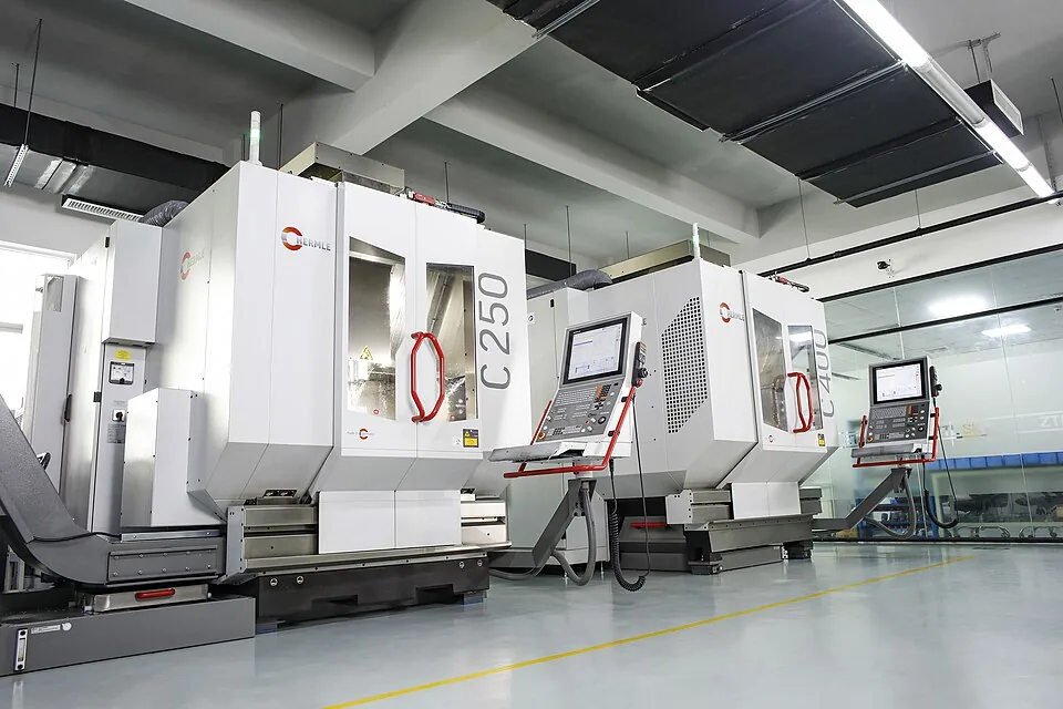
| Type A: Narrow Unimodal Distribution | Twin-pallet horizontal machining centers (HMC) or robotic articulated part loading. | Steep, narrow peak; standard deviation σ < 3 seconds. | Manual intervention occurs completely out of cycle during background pallet indexing. | Predictable throughput; high statistical process capability. |
| Type B: Bimodal Distribution | Manual vertical machining center (VMC); single machinist managing two machines. | Two separate peaks: rapid prompt cycles versus operator-delayed cycles. | Operator occupied at second spindle or detained by benchtop micrometer checks. | The cell toggles across two distinct operational regimes; uncoordinated human-machine interface. |
| Type C: Heavy-Tailed Skewed Distribution | Challenging aerospace alloys (Inconel, titanium); intricate workholding setups. | Low median and mode, but a thick right-hand tail stretching out to 600 seconds. | Stringy chip buildup, feed-hold pauses, probing delays, suspect insert wear, micro-stoppages. | The mean is deceptive; the bulk of lost plant capacity is consumed inside the tail. |
Anatomy of a bimodal distribution: When one machinist tends two vertical machining centers, the process splits naturally. If the machinist is standing ready as Machine 1 completes its program, unloading and reclamping takes 25 seconds, completing the total cycle in 175 seconds. But if the operator is torqueing a vise or deburring a part on Machine 2, Machine 1 sits idle with its doors wide open. Unload-reload balloons to 90 seconds, stretching that cycle to 240 seconds. Combining these groups yields a mathematical mean of 207.5 seconds, yet not a single component in the batch was machined in 207.5 seconds. The distribution exhibits an empty void between two active operating states.[1][7]

Second Critical Insight: Waste Hides in the Tail, Not in the Average
In a 100-piece run where 90 parts complete in 180 seconds and 10 parts stall out to 450–600 seconds, the arithmetic mean settles at approximately 207 seconds. This single metric blends the efficiency of the 90 parts with the severe delays of the 10 parts. When establishing delivery quotes, the decisive question is never “what is the mean duration?” but rather “within what timeframe do 95% of parts finish?” P95 establishes that operational boundary; the remaining 5% tail dictates the safety buffer required in capacity planning.[3][4]
Mathematical Model of Tail Latency Loss
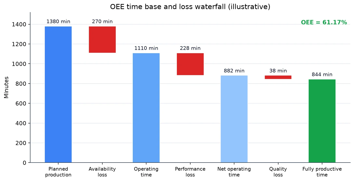
To demonstrate how the arithmetic mean conceals capacity leakage and distorts the Performance component in OEE calculations, let us examine a representative 122-piece production run. This is a controlled mathematical model structured to highlight distribution mechanics:
// 1. Scheduled Shift Time
Shift duration = 8 hours = 480 minutes = 28,800 seconds
Planned downtime (lunch + breaks) = 45 minutes = 2,700 seconds
Net operating time = 26,100 seconds
ERP standard cycle time = 180 seconds
Expected ideal production = 26,100 / 180 = 145 parts

// 2. Actual 122-Piece Batch Telemetry
80 parts × 172 seconds = 13,760 seconds
30 parts × 182 seconds =  5,460 seconds
 8 parts × 300 seconds =  2,400 seconds
 4 parts × 450 seconds =  1,800 seconds
Total machining time ≈ 23,420 seconds

// 3. Derived Distribution Metrics
Arithmetic Mean = 23,420 / 122 ≈ 192.0 seconds
Median (P50) ≈ 173.0 seconds
P90 ≈ 186.0 seconds
P95 ≈ 305.0 seconds
P99 ≈ 453.0 seconds
Capacity deficit = 145 − 122 = 23 parts
Dispersion ratio (P95 / P50) ≈ 1.76
In this model, approximately 90% of the 122 parts finish at or under 186 seconds, which is why P90 sits at 186 seconds. The final 8 parts average 300 seconds, and the slowest 4 average 450 seconds, spreading the tail between 250 and 520 seconds. The 95th percentile threshold lands at 305 seconds because this tail group populates the uppermost 5% bracket of the run. P99 reaches 453 seconds.
A plant manager reviewing the arithmetic mean of 192.0 seconds against the 180-second standard sees only a 12-second variance, which leads to a benign diagnosis of “running slightly below theoretical rate.” Yet the actual capacity deficit of 23 parts does not stem from a mild shop-wide slowdown; it is driven almost entirely by the 12 tail components: 8 × 300 + 4 × 450 ≈ 4,200 seconds. At a standard cycle of 180 seconds, those 4,200 wasted seconds equal exactly 23 parts of unrecovered machine capacity. While the machine runs at peak efficiency for most of the shift, substantial output vanishes in the tail.
This is why P95 is an operational ceiling for scheduling rather than an academic statistic. In an operation where the P95/P50 ratio reaches 1.76, basing quotes on the 192-second average is high-risk; scheduling must reflect the P95 figure of 305 seconds or build an explicit buffer between P50 and P95. The sparse density of columns on the far right of the histogram does not indicate missing data; it reflects the physical reality that in a 122-piece run, the tail consists of just 12 parts. High-resolution continuous distribution curves require 300+ cycles.

Diagnosing Unscheduled Downtime from Distribution Geometry
A cycle time histogram is more than a descriptive summary; it functions as a diagnostic cardiogram of machine health. G-code dwell commands, tool changer indexing stalls, touch-probe calibration delays, and chip conveyor jams do not scatter randomly across time; they imprint distinct geometric signatures within specific duration bands. These signatures allow engineers to diagnose losses that never trigger a machine alarm.[1][3][7]
1. Discrete Secondary Peak (M00 / M01 or Touch-Probe Latency)
A distinct secondary cluster positioned 60–120 seconds above the primary mode typically points to programmed human-machine interaction. Programmed M00 (mandatory program stop) or M01 (optional stop) blocks require operators to open the door, inspect dimensions, flip workpieces, or clear chips. If the operator is attending another spindle, this pause immediately turns into unrecorded idle time. Resolving this profile requires moving to automated in-process probing or decoupled workholding. Micro-stoppage monitoring isolates the duration and frequency of these brief pauses.
2. Right-Skewed Tail (Chip Bird-Nesting and Clearing Delays)
When the right side of the histogram trails off irregularly toward 500–600 seconds, random micro-interruptions are entering the process. In gummy aluminum or soft alloy cutting, stringy swarf wrapping around the toolholder or workpiece forces operators to hit feed hold and clear the nest manually. (Note: Using compressed air guns between telescopic way covers is bad practice; blowing swarf past wipers damages linear guide rails and ballscrews. Cleaning must rely on controlled vacuuming or protective washdown routines.) Because these micro-pauses do not trigger CNC fault codes, standard MES tools miss them entirely, yet they thicken the tail and drag down overall throughput.[7]
3. Periodic Comb Pattern (Tool Life Indexing)
A comb-like pattern where cycle times jump from 180 seconds to 360 seconds at regular intervals—say, every 20 parts—signals scheduled tool life management. When an insert reaches its wear threshold, indexing the tool, clamping fresh carbide, and running a tool-setter touch probe doubles the cycle duration. While this is normal maintenance, grouping this time into part cycle metrics skews capacity calculations; it must be separated into a distinct “periodic tool change allowance.”[6]
4. Rightward Drift Over Time (Thermal Drift and Operator Fatigue)
When median cycle times shift from 175 seconds early in the shift to 188 seconds during the final two hours, process dynamics are changing. This drift stems from two common mechanisms: operator fatigue extending part loading intervals, or spindle/machine thermal expansion prompting machinists to override feed rates downward to prevent dimensional drift. Separating these root causes requires correlating controller sensor logs with operator event timestamps over the shift timeline.[1]
Decision Support Matrix
The thresholds below serve as practical baseline guidelines, subject to calibration based on part geometry, tolerances, and machine age. The objective is not to mandate rigid dogma, but to map observed geometric patterns to targeted engineering actions:[1][7][9]
| Observed Signature | Statistical Trigger | Probable Root Cause | Engineering Countermeasure | Projected Impact |
|---|---|---|---|---|
| Bimodal split (broad mode gap) | Mode 2 − Mode 1 > 45 s; bimodality coefficient > 0.55 | Operator overloaded across multi-machine cell; manual inspection delays. | External setup clamping (SMED), pneumatic quick-point fixtures, or cobot loading. | Merges dual operating modes into single peak; unlocks lost capacity. |
| Elongated right-hand tail | P95 / P50 > 1.50; positive skewness > 1.2 | Chip nesting, chips packing fixture locating pins, inadequate coolant flush. | Chipbreaker insert geometry, modified toolpath engagement, high-pressure through-spindle coolant. | Compresses tail duration; pulls P95 toward P50. |
| Symmetrical wide dispersion | CV > 18%; skewness ≈ 0 | Lack of standardized work instructions; wide variation in machinist habits. | Visual standard work sheets, torque-limiting fixture wrenches, operator training matrices. | Narrows process variance; equalizes output across shifts. |
| Periodic comb spikes | Recurring spikes > 2 × mode at fixed piece intervals | Tool life limit reached; in-cycle touch-probe tool length calibration. | Sister tooling in magazine; automated background tool indexing. | Removes tool indexing from direct cycle time. |
Five-Step Implementation Roadmap
To convert raw cycle time telemetry into reliable production decision tools, adopt this structured five-step engineering roadmap:[1][3][6]
- Capture raw controller timestamps directly: Eliminate paper logs completed at the end of a shift. Stream high-resolution state transitions over MTConnect, FANUC FOCAS, or Heidenhain DNC to capture
Execution(ACTIVE → READY),PartCount, and spindle load signals with millisecond accuracy. For trigger rules, consult the state machine guidelines in our CNC Shift and Part Counting guide. - Decompose cycle time into core components: Avoid logging the entire cycle as an indivisible black box. Split data into in-cut machining time (spindle rotating and axes interpolating) and handling time (door opened → cycle start button pressed). In-cut duration validates cutting parameters and tool stability, while handling time reflects cell ergonomics and material handling efficiency.
- Track P50, P95, and sample volume together: Calculate P50, P90, P95, and P99 for every completed batch. When the P95/P50 ratio exceeds 1.20, trigger an immediate tail loss investigation. For runs under 100 cycles, treat P95 as an exploratory advisory indicator; robust confidence requires 300+ observations.
- Correlate tail cycles with sensor telemetry: For cycles exceeding the P95 threshold, automatically log associated controller states: spindle load alarms, feed-rate potentiometer overrides, door open durations, and probe dwell intervals. This replaces subjective finger-pointing with an objective technical log.
- Publish realistic duration ranges on routing sheets: Replace rigid single-value cycle times on ERP routings with dual parameters:
[P50: 173 s, P95: 305 s]. Calculate scheduling buffers and safety lead times against P95 risk, while using P50 to benchmark pure machine efficiency.
Conclusion: The Average Is Not a Standalone Decision Metric
A CNC facility may appear fully optimized on paper: green lights illuminate machine stacks, and monthly ERP summaries show average cycle times tracking close to nominal benchmarks. Yet if that average masks a volatile mix of 170-second rapid runs and 450–600 second tail delays, substantial plant capacity is silently draining into unrecorded pauses and chip clearing.
The arithmetic mean communicates total machine load, but it explains neither capacity headroom nor delivery predictability. P50 reveals authentic machine capability, while P95 provides the upper limit required for contractual reliability. Reviewing all three metrics simultaneously ensures that engineering, scheduling, and shop-floor operations speak a unified, statistically sound language.
Every manufacturing manager should ask two foundational questions: Does the scheduling system plan around P50, or does it rely on an arithmetic mean that buries the tail? And for parts exceeding P95, how many delays stem from tooling, swarf clearing, probing, or operator logistics—and is the cost of that lost capacity measured?
This article forms the statistical process control and advanced analytics chapter of the DigiLiner CNC Data and Efficiency Series. For machine state categorization in OEE, read How to Calculate OEE in CNC Machining; for losses under five minutes, consult CNC Micro-Stoppage Monitoring; for piece counting state transitions, refer to CNC Shift and Part Counting; and for machine communication protocols, see our comprehensive CNC Control Protocols Guide.
References and Technical Standards
- Douglas C. Montgomery (2012) • Introduction to Statistical Quality Control (7th Edition) • John Wiley & Sons • wiley.com
- Walter A. Shewhart (1931) • Economic Control of Quality of Manufactured Product • D. Van Nostrand Company • asq.org
- ISO 22514-4:2016 • Statistical methods in process management – Capability and performance – Part 4: Process capability estimates and performance measures • ISO OBP — 22514-4
- Sam Savage (2009) • The Flaw of Averages: Why We Underestimate Risk in the Face of Uncertainty • John Wiley & Sons • wiley.com
- ISO 22400-2:2014 • Automation systems and integration – Key performance indicators (KPIs) for manufacturing operations management – Part 2: Definitions and descriptions • cesmii.org
- MTConnect Institute • MTConnect Standard Part 2: Materials Processing – Controller Execution and PartCount Telemetry • model.mtconnect.org
- Modern Machine Shop (Gardner Business Media) • Analyzing Machine Tool Cycle Time Variability and Shop Floor Telemetry • mmsonline.com
- MachineMetrics Inc. • Cycle Time Benchmarks & The Hidden Factory in Precision Machining • machinemetrics.com
- Lean Enterprise Institute • Lean Production Simplified: Cycle Time vs Takt Time and Waste Reduction • lean.org
- NIST/SEMATECH • e-Handbook of Statistical Methods — Percentiles and percentile plots • itl.nist.gov/div898/handbook