




On a typical shop floor, the CAM simulation looks flawless. A 3D machine model rotates on screen, toolpaths flow smoothly, and not a single collision warning appears. Then the same program reaches the machine. During a deep pocket, the cutter starts to chatter, the edge overheats, or the spindle bearings complain. A mold or an aerospace part that took hours to machine can end up in the scrap bin.
The reason is simple: CAM simulation mostly plays back nominal G-code and geometric material removal. It does not know the spindle’s current temperature, the micron-scale growth of a ball screw, how worn the cutter is, or the vibration that appears in the cut. A closed-loop CNC digital twin enters here: not a passive drawing on a screen, but a synchronized representation fed by live telemetry that can act on process parameters within the limits set by the controller and the machine builder. There is no single universal definition, so the level matters.
At a Glance: Closed-Loop CNC Digital Twin Architecture
| Scope | A cyber-physical representation synchronized with a physical CNC machine, processing sensor telemetry and acting on process parameters within permitted limits |
|---|---|
| Logical Layers | (1) Geometry & Kinematics → (2) Process Physics & Thermal Model → (3) Sensing & Telemetry → (4) Closed-Loop Decision |
| Data Direction | Automatic bidirectional: read telemetry from the machine + write permitted parameters (feed, speed, axis offset). Read-only systems are digital shadows; systems without write authority remain at the model or shadow level. |
| Latency Scale | Edge PLC/IPC cycle: 1–10 ms; CNC write path: typically 10–50 ms depending on protocol; thermal correction: 1–5 s; analytics: minutes to hours. The servo torque/current loop closes inside the drive, far faster. |
| Compute Architecture | Deterministic edge computing (DIN-rail industrial IPC, embedded PLC, FPGA where needed) + hybrid cloud for fleet modeling and model training |
| Field Protocols | CNC Control Protocols: FANUC FOCAS, Heidenhain DNC/LSV2, Siemens Sinumerik (OPC UA/Edge), MTConnect, OPC UA |
| International Standard | ISO 23247 series: Parts 1–4 (2021) and Part 5 — digital thread (2026) |
| Core Benefit | Potential to reduce tool breakage and scrap risk; actual gain depends on sensor coverage, model quality, write authority, and part geometry. Vendor percentages are application-specific, not general guarantees. |
There Is No Single Definition of a Digital Twin
The term has become one of the most stretched in engineering. Some vendors call offline CAM simulation a digital twin; some call an OEE dashboard a digital twin; others reserve the label for a closed-loop control system. That inflation muddies investment decisions and vendor comparisons.[1][2]
The most widely cited classification comes from Kritzinger et al. (2018). It looks at whether data flow between the physical system and its digital representation is automatic, and in which direction:[2]
- Digital Model: No automatic data link between the physical and digital sides; data moves by hand.
- Digital Shadow: Automatic, one-way flow from physical to digital; the digital side watches but does not write back.
- Digital Twin (Kritzinger sense): Automatic, bidirectional flow; the digital side can act within permitted limits.
There is an important balance here. Kritzinger’s taxonomy calls bidirectional automatic flow a digital twin, but ISO 23247-1 defines a digital twin as a fit-for-purpose digital representation of an Observable Manufacturing Element (OME) with synchronization between the OME and its representation, and does not require closed-loop actuation.[3][5] So “real digital twin” is a label from a particular taxonomy, not a universal standard. Systems with closed-loop capability are called closed-loop digital twins here.
The Simulation Illusion: Why a Static Model Struggles on the Shop Floor
The most common confusion is treating advanced CAM or VERICUT-style G-code verification as a digital twin. These tools are valuable: they catch collisions, axis limits, and material-removal errors; some even simulate machine kinematics. What they lack is live sensor feedback from the machine on the floor.[2]
This is not just an academic distinction. Siemens positions its digital twin primarily around job preparation, offline programming, and 3D simulation on its SINUMERIK product page.[6] Vendor “digital twin” often means a digital model or shadow; closed-loop control is a separate engineering step. At purchase time, ask two questions: what data arrives automatically, and what parameters are written automatically?
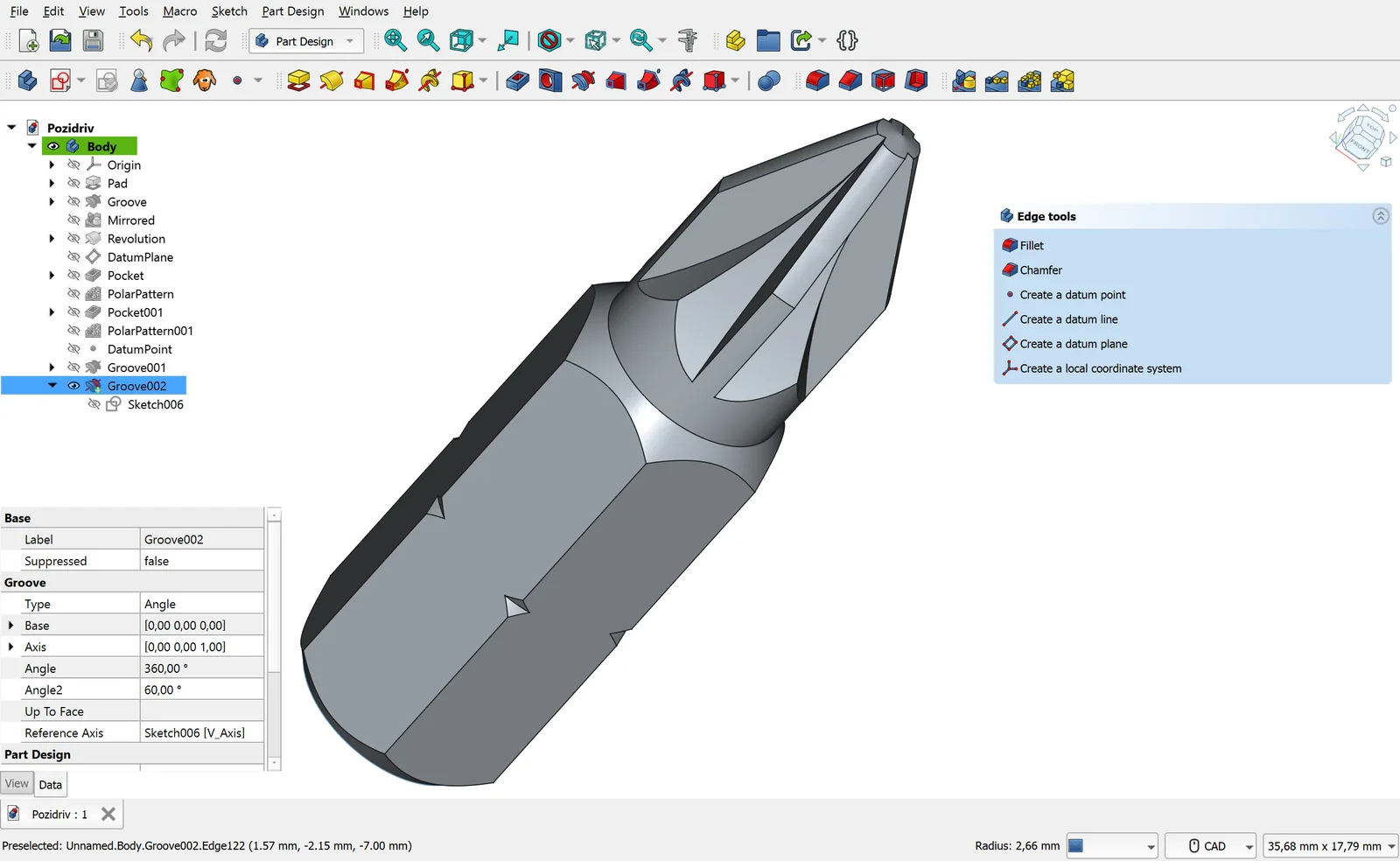
CAM software computes part geometry and the cutter’s theoretical coordinates as a mathematical vector chain. It often assumes the machine structure is rigid, the ambient temperature is constant, the cutter does not wear, and cutting forces can be represented by simplified models. Machining stresses every one of those assumptions.
When the machine starts cutting, a dynamic energy conversion begins. Spindle speed raises friction heat in the bearings; motion along X, Y, and Z engages axial thermal growth in the ball screws. Linear expansion is simple:
ΔL = α · L · ΔT
where ΔL is the elongation, α the coefficient of linear expansion, L the initial length, and ΔT the temperature change. For carbon steel, α is roughly 11.5–12 × 10−6 /K. A 4 K rise over a 1 m structure produces about 46–48 µm of growth.
But place the number correctly. That 48 µm applies to the full meter of travel. Over a 30 mm pocket depth, the screw-related accumulation is about 1.4 µm. Most of the Z-axis error usually comes from thermal growth in the spindle and structure, which can reach tens of microns in the literature.[4] A statement such as “30,000 mm becomes 30,048 mm” is therefore misleading unless the error source and the measurement length are separated. The correct statement depends on which element grows and over what distance.
The second blind spot is cutting dynamics. The Kienzle/Victor model estimates the tangential cutting force semi-empirically:
Fc = kc1.1 · b · h(1−mc)
where Fc is the main cutting force, kc1.1 the specific cutting force for a 1 mm × 1 mm reference chip cross-section, b the width of cut, h the chip thickness, and mc the exponent representing the material’s size effect. kc1.1 and mc vary with material, heat treatment, and tool geometry; a single constant cannot model every material. In milling, helix angle, radial immersion, flute count, and tool wear also enter the picture.[9]
Local hardness variations, tool wear, or a sudden increase in contact length at a corner can spike the force. When those forces coincide with the spindle’s resonance, chatter begins and the cutting edge can fail quickly. A static simulation cannot measure this because it has no live vibration data.
The First Twist: CAM Simulation Is Not a Digital Twin
Sticking a “digital twin” label on a rotating 3D machine animation is one of the industry’s most common mistakes. A CAM or collision-checking package shows the nominal geometric motion of G-code; it is blind to what happens on the floor. A model that receives no data from the machine, sees no worn tool, no expanding ball screw, no warming spindle bearing, is a static digital model, not a twin. That does not make simulation worthless: it is essential for collision prevention and first-pass program verification. A digital twin does not replace simulation; it feeds simulation with live data.
The Three-Step Evolution: Digital Model, Digital Shadow, Closed-Loop Twin
The table below summarizes three levels based on data flow. This is not a maturity pyramid; each level serves a different need.[2][3]
| Feature / Level | Digital Model | Digital Shadow | Closed-Loop Digital Twin |
|---|---|---|---|
| Physical to Digital | Manual (human input) | Automatic (sensor / telemetry) | Automatic (live and high-speed) |
| Digital to Physical | Manual (USB / DNC transfer) | None (monitoring only) | Automatic, limited to permitted parameters |
| Timing | Offline (design time) | Near real time (typically 1–5 s dashboard latency) | Edge PLC/IPC cycle 1–10 ms; CNC write path 10–50 ms depending on protocol |
| Critical Hardware Location | Engineering workstation | Plant server / cloud | Shop-floor edge device (Edge IPC / PLC) |
| Typical Industrial Example | SolidWorks, Mastercam, NX CAM | Grafana, SCADA dashboards, OEE monitors | Siemens SINUMERIK ONE, Beckhoff TwinCAT 3, Caron TMAC |
“Closed loop” in this table does not mean every machine parameter can be changed freely. In practice, write authority is bounded by the CNC interface the builder exposes, the PLC program, the safety interlock, and the parameter limits the machine builder approves. A closed-loop twin is not an autonomous black box; it is an auditable engineering system.
The Second Twist: “We Built a Digital Twin” Usually Means a Digital Shadow
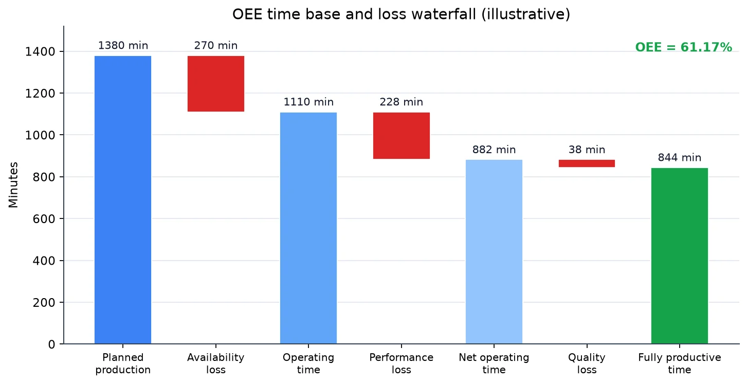
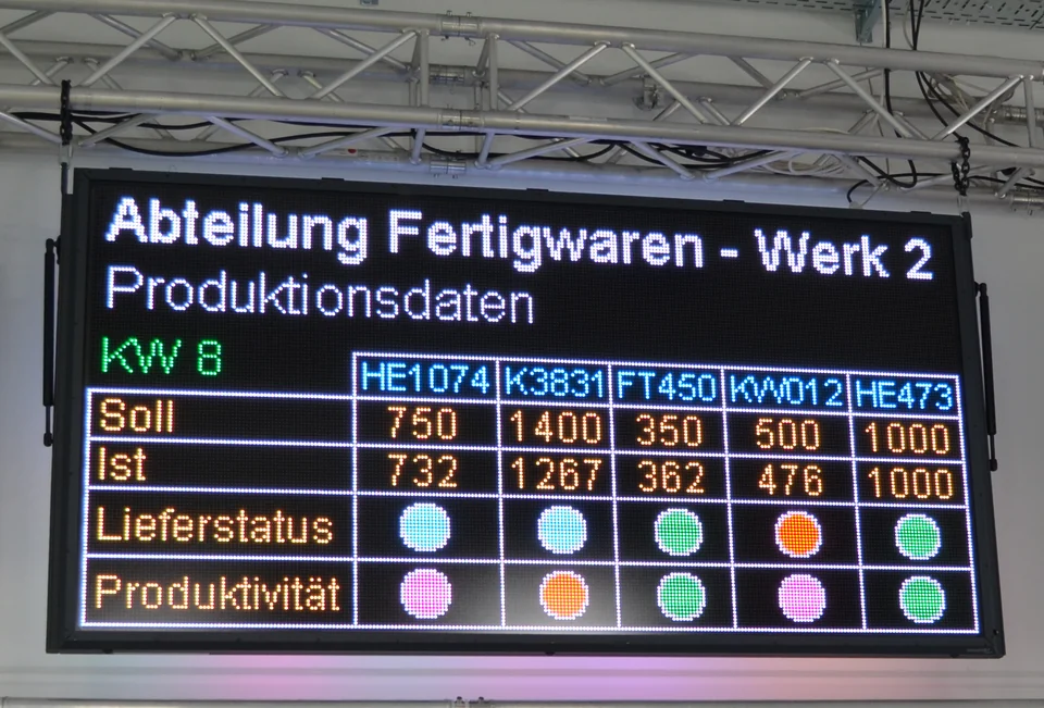
Pushing machine data into colorful charts, tracking part counts or spindle load remotely is valuable operational capability, but the communication is a one-way monologue. If a human sees tool wear on screen and presses stop, you have a digital shadow, not a Kritzinger digital twin. That does not make it useless: OEE, energy, and downtime analysis are exactly what most factories need. Closed loop should be justified only for high-risk or high-value parts.
The Four Logical Layers of a CNC Digital Twin
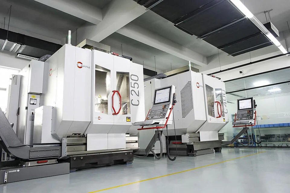
A comprehensive CNC cyber-physical twin architecture rests on four logical layers. They are an engineering distinction, not a standard.[3] Five-axis machines make the kinematic layer concrete: Hermle, for example, describes the C 250 GEN2 as its entry model into 5-axis milling.[11]
1. Geometry and Kinematics (Spatial Verification)
This layer defines the machine’s physical kinematics and structural volume. The A and C rotary tables of a five-axis machining center, linear guides, tool holders, fixture clamps, and the raw stock are represented in three dimensions. The live axis coordinates from the controller’s interpolator (X, Y, Z, A, C) are processed through kinematic transformations. The layer’s primary job is collision prevention, axis-limit enforcement, and tracking the tool tip’s instantaneous vector position relative to the part.
2. Process Physics and Thermal Model
This layer puts the physics of machining inside the geometric model. Two critical models run here:[4][9]
- Force and Vibration Model: Instantaneous cutting forces are estimated from the cutter edge geometry, helix angle, the workpiece material’s specific cutting resistance, and the Kienzle/Victor approach. Frequency response functions (FRFs) from a modal test of the machine are added to produce stability lobe diagrams. The model tries to predict the speed and depth of cut at which the machine will enter resonance (chatter). That prediction must be recalibrated for every machine-tool combination.
- Thermal Deformation Model: Ambient temperature, spindle bearing temperature, and linear scale data are used to map the growth of the machine structure and ball screws. As the machine warms up, the resulting Z-axis drift is calculated and sent to the CNC offset table. Accuracy here depends on sensor placement and model calibration; there is no guarantee that “I measured the temperature, so the thermal error is solved.”
3. High-Speed Sensing and Telemetry
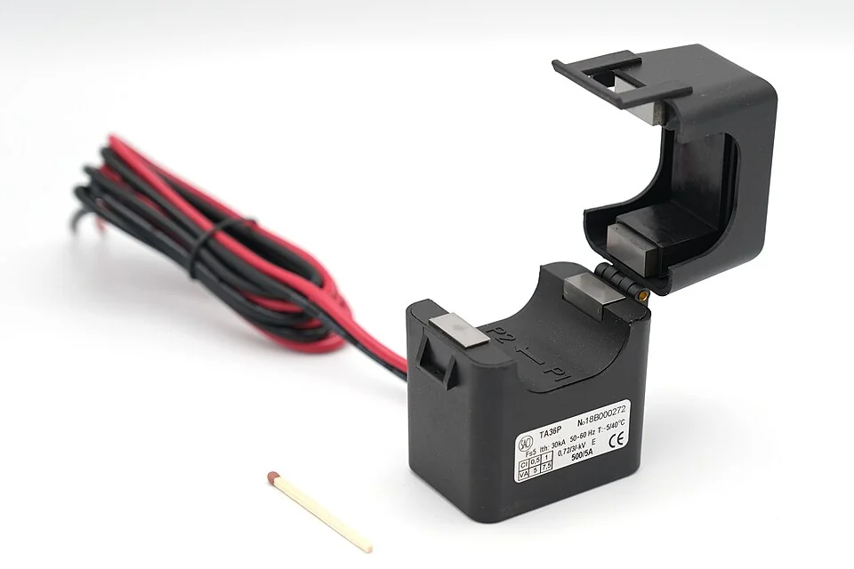
The controller’s standard interpolator cycle is typically 1–4 ms on modern CNCs; older systems can be slower. To capture cutting dynamics, external high-speed sensors are also needed. Piezoelectric accelerometers on the spindle and Hall-effect current sensors or split-core current transformers can be added to an older machine.
Do the sampling math correctly. For a milling cutter, the tooth-pass frequency with spindle speed n (rpm) and z flutes is approximately ft = z · n / 60. A four-flute cutter at 20,000 rpm has a tooth-pass frequency of 4 × 20,000 / 60 ≈ 1.333 Hz. The Nyquist criterion requires sampling at least twice the highest frequency of interest, so the theoretical floor is about 2.7 kHz. In practice, 10–50 kHz is often chosen for anti-aliasing, impact content, and chatter sidebands. Saying “Nyquist requires at least 10 kHz” is technically wrong; 10 kHz is an engineering margin, not a Nyquist requirement.[8]
As an industrial example, Caron TMAC specifies vibration measurement up to 22 kHz and a power sensor sampling rate of 256,000 samples per second; it claims a 5 ms response to tool breakage.[8] Such vendor claims are useful for understanding the achievable order of magnitude, but they do not guarantee the same result in every application.
4. Closed-Loop Decision Layer
This is where the layers converge and become action. Live torque and vibration data are compared with the physical cutting model. When the model determines that “expected torque is 12 Nm, measured torque is 26 Nm; the tool tip is about to break or the tool is severely worn,” a millisecond-scale intervention is triggered. The action can write “Feed Hold,” “Adaptive Feed Override,” or “Spindle Speed Modulation” to the PLC through a Unified Namespace (UNS) or a real-time fieldbus bridge (EtherCAT / Profinet). The write is limited to the parameters the controller and machine builder permit; the safety PLC, interlocks, and relevant machine-safety standards (e.g., ISO 13849 / IEC 62061) remain in force. On the industrial cybersecurity side, the IEC 62443 framework should be considered.
One distinction matters: the servo motor’s torque/current loop closes inside the drive at a much higher rate. The edge IPC or digital twin software usually does not replace that inner loop; it makes decisions at the process level (feed, speed, tool change, thermal offset). “The digital twin controls everything in microseconds” is therefore not a realistic claim.
The Cloud Latency Wall: Why Edge Computing
Cloud computing is strong for fleet-wide analytics, cross-machine wear models, and ERP integration. But when the subject is the physics of chip removal, a cloud architecture is not suitable for a deterministic control loop.[5][7]
Time moves differently in machining. At 18,000 rpm with a four-flute end mill, each edge enters and leaves the material about 1,200 times per second. Depending on immersion, a single edge can be in cut for roughly 0.2 ms. Chip jamming, a hard inclusion, or resonance building into destructive chatter can happen in a few milliseconds to tens of milliseconds. Commercial tool-monitoring systems such as Caron TMAC aim for a 5 ms response.[8]
Cloud latency depends on distance, network load, and carrier. A round trip to a cloud region in the same city can be a few milliseconds to 20 ms; over the public internet or remote regions it can exceed 50–200 ms; cellular links can show 20–100 ms. These are orders of magnitude, not guarantees. The defensible statement is not “80–250 ms even on perfect fiber,” but “the cloud offers no deterministic upper bound.”
The Third Twist: The Cloud Is the Twin’s Memory and Training Ground, Not Its Brain
Sending sensor data to the cloud while the machine cuts at 18,000 rpm, running a model there, and sending a “stop” command back is not hard real-time control. Tool breakage can occur in a few milliseconds; a cloud round trip can take tens to hundreds of milliseconds. The critical decision engine must therefore live on the edge processor at the machine. The cloud aggregates fleet data, trains models, and distributes updated parameters to the edge. The cloud is not “never used”; it is not used in the hard real-time inner loop.
This physical constraint drives modern cyber-physical systems toward a two-tier hybrid architecture:[5][7]
- Edge Layer (deterministic decisions): Industrial PCs tied directly to the PLC cycle (for example, Beckhoff IPC/TwinCAT 3, edge solutions around Siemens SINUMERIK ONE, or tool-monitoring systems such as Caron TMAC). These devices can respond at 1–10 ms at the process level; adaptive cutting-force control and instant tool protection are decided locally. If a CNC interface write is required, the path is typically 10–50 ms depending on protocol.
- Cloud Layer (strategic learning): Collects filtered data from dozens of machines. It analyzes which tool geometry lasts longer in which batch, trains fleet-level predictive-maintenance models, and distributes updated weights to edge devices during night shifts.
Decision-Support Matrix: Which Process Needs a Digital Twin?
A genuine closed-loop digital twin is a serious engineering investment: external sensor infrastructure, high-speed edge hardware, machine kinematics modeling, and controller write permissions. Applying a full twin to every machine and every part is an economic mistake. The matrix below is a starting point for matching process complexity with the right digitalization level:[2][5]
| Manufacturing Type & Part | Typical Risk & Cost of Failure | Required Level | Investment Rationale |
|---|---|---|---|
| Aerospace & Defense: titanium and nickel-based superalloy fan/compressor components, thin-walled structures | Very high: part cost and machining time are high; a single tool break can scrap an expensive part. | Closed-loop twin or high-speed adaptive control | Thermal compensation, chatter suppression, and tool-break protection. ROI must be calculated per part and against scrap cost; there is no general “six-month payback” guarantee. |
| Large automotive press dies and injection molds | High: large press dies can weigh tens of tons; injection molds are usually smaller. Losing surface form means long manual correction. | Thermal drift + vibration suppression (closed loop or advanced shadow) | Confidence for long finishing operations and unattended/night machining. A generic “3× spindle life” claim should be replaced by measurement on your own machine. |
| Precision medical implants (titanium spinal screws, knee prostheses) | Medium-high: FDA UDI (21 CFR Part 830), Quality System Regulation (21 CFR Part 820), and ISO 13485 traceability; micron-level surface quality is critical. | Advanced digital shadow + hybrid adaptive control | Part-level production records and process traceability. Inspection-cost gains are possible, but the rate varies by application. |
| High-volume serial production (automotive bushings, standard flanges, bolts) | Low-medium: unit price is low, operations are short, and the machine setup is usually stable. | Digital shadow (OEE, downtime, energy) | A full closed-loop twin is often over-engineering. A standard MTConnect/OPC UA telemetry path and an OEE dashboard are enough in most cases. |
| General contract machining (small-batch job shop) | Variable: materials and parts change constantly; engineering budget per machine is limited. | Digital model + advanced CAM simulation | Verified CAM simulation and an accurate tool library are the first rational step to prevent basic collisions. Closed-loop investment makes sense only for repeat, high-value work. |
This matrix is a framework, not a recipe. A real ROI calculation must include part geometry, machine age, existing sensor infrastructure, scrap and rework cost, labor and energy cost, and software maintenance. Vendor case-study percentages cannot be generalized without a baseline measurement on your own line.
ISO 23247: A Shared Framework and Its Limits
For years, proprietary ecosystems were the biggest obstacle to multi-brand digital twins. Each CNC brand pushed its own interface—FANUC FOCAS, Heidenhain DNC, Siemens Sinumerik—making a single central twin hard in a mixed shop. ISO 23247 offers common terminology and a reference architecture, but it is not plug-and-play.[3][5]
The ISO 23247 series (“Automation systems and integration — Digital twin framework for manufacturing”) consists of:
- Part 1 (Overview and General Principles, 2021): Defines basic terms, terminology, and general requirements.
- Part 2 (Reference Architecture, 2021): Defines four domains—observable manufacturing, data collection and device control, core, and user—and five entities: the Observable Manufacturing Element (OME), Data Collection and Device Control Entity (DCDCE), Core Entity (CE), User Entity (UE), and Cross-System Entity (CSE), which provides shared functions across systems.
- Part 3 (Digital Representation of Manufacturing Elements, 2021): Describes basic information attributes for OMEs and which existing standards can be used, such as IEC 62264-2 for enterprise-control integration.
- Part 4 (Information Exchange, 2021): Defines information-exchange requirements for user, service, access, and proximity networks. It does not mandate a single protocol; in practice, open standards such as MTConnect, OPC UA, and MQTT are widely used.
- Part 5 (Digital Thread for Digital Twin, 2026): Defines how the digital thread connects, manages, and sustains digital twins across the product lifecycle.
With this framework, raw signals from different controllers can be mapped into a common information model. In practice, each brand still needs a profile or mapping. ISO 23247 conformity is not a certificate; it is a design and integration discipline. Combined with a CNC data pipeline and a Unified Namespace, a digital twin can make the whole shop’s machining ecosystem visible, not just one machine.[10] For the protocol layer, see the CNC control protocols guide and What Is MTConnect?.
Closing: Two Questions for a Live Copy
The value of a CNC digital twin is not the resolution of the animation on screen; it is which decision it can make while the tool is in the cut, how much latency it has, and within what safety limits. But do not overstate it: the right level for many factories is a well-designed digital shadow or a verified CAM simulation, not a closed-loop twin.
Ask two concrete questions at the machine:
- Monologue or dialogue? Does the model only watch the physical world, or can it act on the controller within permitted limits and reduce feed before a tool breaks?
- Where is the decision made? Do the algorithms that prevent tool breakage and resonance wait in a cloud server with unpredictable latency, or do they run in a deterministic edge processor close to the physics?
Perhaps the maturity of a CNC digital twin is measured not by how many sensors it connects, but by how clearly it defines which data it uses, for what purpose, and within which limits it turns that data into action.
References
- [1] Michael Grieves & John Vickers (2017) • Digital Twin: Mitigating Unpredictable, Undesirable Emergent Behavior in Complex Systems • Springer, DOI: 10.1007/978-3-319-38756-7_4
- [2] Kritzinger, W., Karner, M., Traar, G., Henjes, J., & Sihn, W. (2018) • Digital Twin in manufacturing: A categorical literature review and classification • IFAC-PapersOnLine, 51(11), 1016–1022 • doi.org/10.1016/j.ifacol.2018.08.474
- [3] ISO 23247 series • Automation systems and integration — Digital twin framework for manufacturing • Part 1: ISO 23247-1:2021 • Part 2: ISO 23247-2:2021 • Part 3: ISO 23247-3:2021 • Part 4: ISO 23247-4:2021 • Part 5: ISO 23247-5:2026
- [4] Mayr, J., Jedrzejewski, J., Uhlmann, E., Alkan Donmez, M., Knapp, W., Härtig, F., Wendt, K., Moriwaki, T., Shore, P., Schmitt, R., Brecher, C., Würz, T., & Wegener, K. (2012) • Thermal issues in machine tools • CIRP Annals, 61(2), 771–791 • doi.org/10.1016/j.cirp.2012.05.008
- [5] National Institute of Standards and Technology (NIST) • Use Case Scenarios for Digital Twin Implementation Based on ISO 23247 • NIST AMS 400-2 • doi.org/10.6028/NIST.AMS.400-2
- [6] Siemens Digital Industries • SINUMERIK CNC — digital twin, offline programming, and 3D simulation • siemens.com/global/en/products/automation/systems/cnc-sinumerik.html
- [7] Beckhoff Automation • TwinCAT 3 — PC-based real-time control, PLC/NC/CNC, and OPC UA • beckhoff.com/en-en/products/automation/twincat/
- [8] Caron Engineering • TMAC — Tool Monitoring Adaptive Control (5 ms response, 22 kHz vibration, 256 kS/s power sampling) • caroneng.com/products/tmac/
- [9] Sandvik Coromant • Specific cutting force (kc1) and the Kienzle/Victor approach • sandvik.coromant.com/en-us/knowledge/materials/specific-cutting-force
- [10] MTConnect Institute • Machine Tool Semantic Data Architecture & Interoperability • mtconnect.org
- [11] Maschinenfabrik Berthold HERMLE AG • Machining centre C 250 GEN2 — entry model into 5-axis milling • hermle.de/en/machining-centres-automation/models/machining-centre-c-250-gen2/